How to Effectively Sum a Column in Excel for Enhanced Data Analysis in 2025
Excel is a powerful tool for data management and analysis. An essential skill for anyone using Excel is the ability to calculate the sum of a column. This capability can greatly enhance your data analysis tasks, whether you are working with financial reports, organizing data entries, or conducting overall assessments of your worksheets. In this article, we will explore various techniques and tips to effectively sum a column in Excel while improving your overall efficiency and productivity.
Understanding the Basics of Excel Summation
To get started, it’s crucial to understand what summation means in the context of Excel. Summation refers to the process of adding a range of numerical values contained within the selected cells of a column. Excel provides a user-friendly interface with built-in functions for this very purpose, making it straightforward to perform addition operations. To calculate the total of a column, you can use specific formulas or utilize the Auto-Sum feature available in the toolbar. Mastering this skill can allow for more accurate calculations and data representation.
Using Basic Formula for Summation
One of the most fundamental ways to sum a column is by using the basic SUM function. To do this, start by placing your cursor in the cell where you want the total to appear. You can then enter the formula as follows: =SUM(A1:A10), where A1:A10 is the range of cells you wish to total. This method automatically calculates the total for all numeric values in that range. It’s an effective way to combine **addition** functionality with flexibility, allowing you to adjust the reference range as needed.
Exploring the Auto-Sum Feature
The Auto-Sum feature in Excel is a time saver that allows you to sum a column quickly with just a few clicks. To use it, select the cell directly below your column of numbers and click on the Auto-Sum icon in the toolbar. Excel will automatically detect the adjacent cells and propose a range to sum. You can confirm its selection or adjust it if necessary before pressing Enter. This feature is especially helpful for rapid summation of extensive data entries, enhancing your spreadsheet’s performance while maintaining accuracy.
Utilizing Shortcuts for Quick Calculations
Excel is also packed with shortcuts that can streamline your summation process. For example, after highlighting a column of values, you can simply press Alt + = on your keyboard to activate Auto-Sum, producing immediate results. This optimization contributes significantly to productivity by reducing the time spent searching for menu items. Familiarizing yourself with these shortcuts will allow for more efficient worksheet management, especially during periods of heavy data manipulation or financial analysis.
Advanced Techniques for Summation
While basic summation skills are crucial, advanced techniques can provide even greater data insights. Excel’s versatile functions allow for conditional sums, dynamic references, and multi-range calculations. Learning to utilize these features not only enhances your analytical capabilities but also helps you display complex data effectively.
Conditional Sums with SUMIF
For scenarios where you need to sum values conditionally, the SUMIF function is invaluable. This function allows you to sum cells based on a specified condition. For example, if you want to total only the sales figures greater than a specific threshold, your formula would look something like =SUMIF(B2:B10, “>1000”). This function is ideal for financial reports or any analysis that requires filtering out specific data entries based on performance criteria, ensuring that your summation aligns with your overall data analysis goals.
Using Dynamic Ranges for Improved Calculations
Dynamic ranges improve the flexibility of your Excel worksheets by automatically expanding or shrinking based on data changes. To create a dynamic range for summation, you could define a named range using the OFFSET function, which allows you to sum a column that frequently changes. For instance, with =SUM(OFFSET(A1,0,0,COUNTA(A:A))), you can dynamically calculate the total for entries in a specified column without needing to adjust the formula manually each time you add new data entries. This method significantly increases accuracy and improves the overall efficiency of your Excel operations.
Understanding Cell References for Accurate Calculations
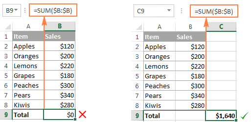
Understanding how to manipulate cell references can enhance your proficiency in Excel. For example, using relative, absolute, and mixed references in your formulas will lead to more accurate calculations. To use an absolute reference while summing, you can lock a specific cell using the $ symbol, such as =SUM($A$1:$A$10). This adjustment ensures that as you copy the formula to other cells, the reference remains constant, which is essential for consistent calculations across a large set of data.
Visualizing Data Aggregation in Excel
Summing columns in Excel is not just about calculation; it’s also about how you visualize the aggregated data. Creating charts or utilizing pivot tables can help you make sense of large data sets, providing clarity and insight, particularly in financial analysis. Highlighting totals can improve reporting capabilities and data storytelling.
Creating Charts for Summed Data Visualization
Once you have summed a column, consider visualizing your data using Excel’s charting features. Charts allow you to present your summed totals in a visually appealing manner, helping to demonstrate trends and patterns in your data analysis. For instance, if you have monthly sales data, summing each month and displaying it in a bar graph can help stakeholders quickly grasp performance trends over time. The capacity to visualize summed data not only enhances your presentations but also improves data communication across teams.
Utilizing Pivot Tables for Advanced Summarization
Pivot tables are powerful tools that enable you to aggregate and analyze your data efficiently. After summing up various data points, you can create a pivot table to summarize these figures dynamically. By dragging and dropping fields, you can organize entries based on categories, providing a comprehensive view of your data analysis. This feature is particularly advantageous for handling large datasets, allowing you to extract meaningful insights quickly. To create a pivot table, select your data range, go to the Insert tab, and choose Pivot Table. From there, begin your analysis effortlessly.
Tips for Effective Data Formatting and Display
You can enhance the clarity of your summed data by applying proper cell formatting within Excel. To do this, ensure appropriate number formatting for currency, percentages, or decimal places, enhancing readability and comprehension for your audience. Furthermore, utilizing conditional formatting features can allow you to highlight specific totals or entries that meet certain criteria, making your worksheet not only functional but visually appealing as well. These enhancements can significantly uplift the overall user interface of your reports, increasing their impact.
Summary of Best Practices for Summing in Excel
In conclusion, summing a column in Excel is an essential skill that lends itself to effective data analysis. From basic functions like SUM to advanced features like conditional sums and dynamic ranges, understanding how to capitalize on these tools will improve your productivity and the accuracy of your calculations. Visualizing your summed data with charts and pivot tables further enhances your reporting capabilities. Mastering these techniques is crucial for anyone looking to harness the full power of Excel in data analysis in 2025.
FAQ
1. What is the fastest way to sum a column in Excel?
The quickest method to sum a column in Excel is by using the Auto-Sum feature. Simply click on the cell below your numerical data, go to the toolbar, and select Auto-Sum. This feature automatically suggests a range to sum, saving you time on manual input.
2. Can I sum non-contiguous cells in Excel?
Yes, you can sum non-contiguous cells using the SUM function by including the cells separated by commas. For example, =SUM(A1, A3, A5) will total the selected non-contiguous cells directly.
3. How do I sum a column based on criteria?
To sum a column based on specific criteria, use the SUMIF function. The syntax is =SUMIF(range, criteria, [sum_range]), allowing you to filter the entries that meet your specified conditions effectively.
4. How do I sum a column automatically when new data is added?
You can use a dynamic range formula like =SUM(OFFSET(A1, 0, 0, COUNTA(A:A))) to ensure that the summation automatically adjusts when new entries are added to the column.
5. What’s the benefit of summing values visually in a chart?
Summing values and displaying them in a chart provides a visual representation of data trends, making it easier for stakeholders to understand performance at a glance. This enhances data communication and helps drive insights from the aggregated data more effectively.
6. Can Excel sum text values?
Excel cannot sum text values directly. If the text entries in a range are numeric, make sure they are formatted correctly as numbers. If they’re stored as text, you can convert them using a VALUE function to enable summation.
7. What formatting options enhance the clarity of summed data?
Utilizing number formatting (for currency or percentages), conditional formatting (to highlight important figures), and clear column headings can significantly enhance the clarity of summed data in Excel, improving the overall presentation of your spreadsheet.